Introduction
So, a few days ago a colleague at work said he has been studying
Elliptic Curve Cryptography (ECC) and went to ask me if his
understanding of the ECDSA [1] was
correct. Getting caught by surprise I (first had to refresh my
memory 😅 as its been a while since the last time I actually looked
at the algorithm inner workings, then I) tried to explain the
algorithm verbally with some improvised drawings. He seemed to
understand that his previous idea of the algorithm was almost
right, but not quite there, however, I think I may have left him
more confused than before.
Later that same day, I tried to find some resources that I could send him to clarify what the algorithm was doing. To my surprise, I didn’t find any resources remotely close to what I wanted. Every post/tutorial/video I found on ECDSA followed the same pattern:
- explain graphically what elliptic curves are
- explain graphically Point Addition and Point Doubling
- explain algebraically the ECDSA
tell some big story about how great the bitcoin security is because of the ECDSA
As you can see from the points above, the usual approach consists of “explaining the foundations of ECC” graphically, then explaining the actual ECDSA algebraically. This can be a logical gap for some people, as the base ideas around Elliptic Curves are explained all visually, but when it comes to the actual signature part, we just simply tell you to follow this “equation recipe” and that “the signature will work”.
To redeem myself with this colleague for my bad improvised
explanation, in this post, I’ll try to fill this logical gap and
hopefully, also make it easier for other people that might have the
same problem understanding the algorithm in the “usual way”.
To be clear, I’m not against teaching the ECDSA in the way textbooks show it. I also learned it in the same exact way and never actually thought about it up until this colleague approached me. What I’ll try to bring here, is a bit of an intuition of what the ECDSA is doing and why it works in the way it was designed.
Refresher about the ECDSA 🍹
Before trying to explain the ECDSA visually, let me give you a brief refresher of the ECDSA algorithm “in the usual way” (in other words, let me also contribute to the pool of “explaining ECDSA algebraically” on the internet). As there are plenty of resources available on the web, I’ll try to be brief here (knowing myself, it will probably not be as brief as I originally wanted, but I’ll try 😬).
Elliptic Curves
Elliptic curves are, as the name implies, curves on the 2D plane, described by its characteristic equations. The equations on the other hand, are not ellipses as you might be inclined to think due to their name (the naming actually comes from the fact that they have a close relation to the equations used to calculate the arc length of an ellipse).
The most common representation for an elliptic curve (at least in
introductory cryptography classes) is what is called the
Weierstrass form gosh, I really hope I wrote his name
right. This form is normally presented by the Equation
\ref{eq:weierstrass}:
\begin{equation} \label{eq:weierstrass} y^2 = x^3 + ax + b \end{equation}
An example of the plot for the above equation can be seen on Figure 1:
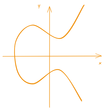
Figure 1: Example of an elliptic curve in Weierstrass form
Elliptic Curves as a Group
Now some readers might be thinking:
Okay, elliptic curves are… curves…, on the 2D plane, but what does this even have to do with cryptography?
That’s when the fun part begins…
On top of the base definition of it being a… curve 🤷, cryptographers and mathematicians also added a set of “rules” over them to make them useful, similar to what we would do to create a board game.
For instance, in a game of chess, pieces can only move a certain way and they cannot move out of the board (unless they are captured). These set of rules define what can and cannot be done within a game of chess. If chess can have its set of rules, why can’t we have our own over the elliptic curves?
These rules “added” to the elliptic curves allow us to consider it a “group” (i.e. group in the mathematical sense, where it follow a series of formal definitions that I’m not going to enter in details here as it is not the scope of this post). This group definition defines how operations are made on an elliptic curve and how the elements inside should behave (also considering edge cases).
There is an algebraic description for these “rules”, but as I intend to explain the ECDSA visually later, the geometric interpretation should be enough for us (also, it is what the majority of posts on the internet show as well).
To define a (mathematical) group, over the elliptic curves we need to define at least three things:
- an operation (here we will define the operation “addition”)
- a neutral element
- an inverse element
Using all of these properties, we can define how to operate over the elements and how they should behave inside an elliptic curve. What is meant by “element”, is just a point \((x, y)\) that satisfies the curve equation (in other words, it is a point inside the curve), as shown in the Figure 2.
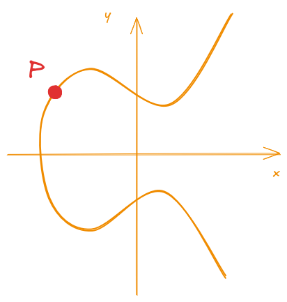
Figure 2: Representation of an element (point P) inside an elliptic curve
Point Addition
The geometric interpretation of the point addition inside an elliptic curve can be described by some “steps”.
To perform the addition of two distinct points \(P\) and \(Q\), it is necessary to:
- trace a secant line that passes through \(P\) and \(Q\)
- check where does the secant intersect on the curve besides \(P\) and \(Q\)
- find the symmetric point to the intersection with respect to the \(x\) axis
Visually, these steps are demonstrated in Figure 3.
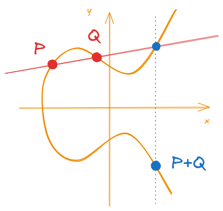
Figure 3: Example of a point addition over an elliptic curve
Naturally, we can also use the same steps if we want to perform an addition of the same point with itself (i.e. \(P + P = 2P\)). The only difference is that the secant will turn into a tangent. This is called point doubling and it is illustrated in Figure 4.
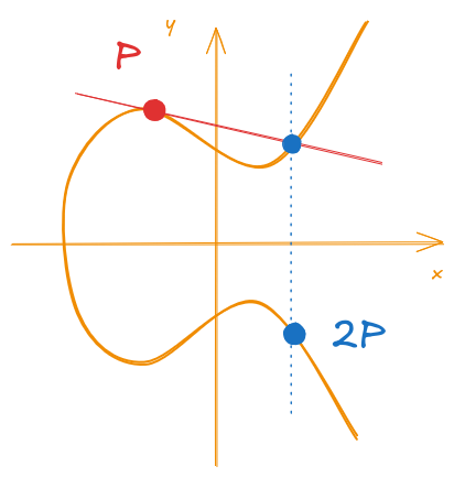
Figure 4: Example of a point doubling over an Elliptic Curve
With point addition and point doubling, we can now perform any arbitrary scalar multiplication over the points.
For example, if we wanted to calculate 3P, we can do it by calculating 2P + P, where we get
the 2P from point doubling.
With that, we could for example, calculate any (scalar) multiplication like 35P, with only
these two operations.
This is actually where the security of ECC comes from. Given that it is easy to “go forward”
(e.g. from a point P to go to 35P), but it is actually hard to “go back” (e.g. from 35P
to P). This is because, since the operations are not linear, if I give you two points P
and Q and asked you, “how many times did I multiplied P to get Q”, you cannot simply
divide one by another to get the result. This kind of property of “going one way” is what we
call a “trapdoor function” in cryptography.
Okay, I should make a little note here about trapdoor functions on ECC.
When we talk about trapdoor functions in cryptography, we are dealing with computationally hard problems to solve. That’s the reason why a lot of cryptographic algorithms deals with prime numbers, as prime numbers have a lot of nice properties that are hard to solve.
For the case of elliptic curves, the “going one way” I told you is actually simple to solve when we are dealing with curves over the real domain. The problem only becomes hard when we use curves over finite fields (I’ll be touching on what’s that later on). This hard problem on elliptic curves is what is called the Elliptic Curve Discrete Logarithm Problem (ECDLP), and you should focus on the word Discrete here.
So while I’ll be approaching the curves on the real domain in this post to bring a better intuition, the actual security of the scheme only happens when we deal with finite fields curves.
Neutral Element
Another property of a mathematical group is the definition of a neutral element for the operation. This is an element that, when operated on, doesn’t change the result. For natural numbers over the addition, this element is the number 0, because adding anything to 0 still gives us the “anything” (i.e. the other value).
On elliptic curves, there isn’t actually an element inside the curve that satisfy this requirement, but as we need them to construct a group, we then define this point as what we call a point at infinity \(\mathscr O\). This point can be visualized as a “point” that is located at \(y = +\infty\) or \(y = -\infty\).
This point, as per definition, should satisfy that:
\begin{equation} \label{eq:point_at_infinity} \mathscr O + P = P + \mathscr O = P \end{equation}
Inverse Element
With the Neutral Element defined, we can now define the final property: the Inverse Element. This property defines that all elements in the group should have an inverse. By inverse, what it is meant is an element that, when operated with the original element, should result in the Neutral Element. In other words, an inverse element (\(-P\)) should satisfy that:
\begin{equation} \label{eq:inverse_element_def} P + (-P) = \mathscr O \end{equation}
Luckily for us, the inverse element is pretty simple when we are dealing with elliptic curves. The inverse for a point \(P = (x_p, y_p)\) is simply:
\begin{equation} \label{eq:inverse_element_of_p} -P = (x_p, -y_p) \end{equation}
Graphically, the inverse is the symmetric point in relation to the \(x\) axis. This is illustrated by Figure 5.
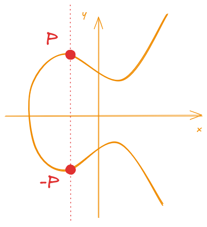
Figure 5: Inverse Element of the point P
ECDSA
With all of the definitions for the elliptic curves as a group, we can now utilize it as a tool to build the actual signature scheme: ECDSA (Elliptic Curve Digital Signature Algorithm).
For this explanation I’ll be using the following parameters/notation:
- an elliptic curve E
- proper coefficients a and b
- modulus p
- a base point G
- order of the subgroup n (generated by G)
Okaaaay, that’s a lot of information for someone that never studied elliptic curves and I also didn’t explained these either on the last section, but there is a reason why.
In the last section, I explained elliptic curves over the real
domain, that’s why the figures were pretty to plot. However, in
real cryptographic applications, we don’t use real numbers,
instead, we either use binary or prime curves over finite fields
(if you never seen this fancy term before there is a first time
for everything, don’t worry too much about it, think of as another
way of doing math using integers and modular arithmetic).
As this post is about “Visualizing the ECDSA”, I intend to also explain those with images, so I’ll use the real domain curves and not the finite fields ones. The reason I’m showing these parameters now is only because I’ll show the actual equations that define the ECDSA.
To expand a bit on the parameters and not just “throw them at your face”, here is a bit on each of the parameters:
The elliptic curve E and the coefficients a and b are just the parameters that define which curve we are going to use. Remember that an elliptic curve is defined by an Equation of the type:
$$y^2 = x^3 + ax + b$$So different parameters define different curves. Just as a curiosity, I won’t show it here, but if you search on the web, there are a lot of interactive sites that you can play with the coefficients and see their impact on the final curve.
The modulus p is actually a “new” parameter if you didn’t study ECC before.
It is not that necessary for what I’ll be explaining later but, as I mentioned, in cryptography we actually use finite fields and, because of that, a modulus always “follow” the original equation (that’s what makes finite fields… finite). With this modulus, the Equation \ref{eq:weierstrass} in finite fields is actually:
$$y^2 = x^3 + ax + b \mod{p}$$A modulus operation, if you never seen one, is just the calculation of the remainder over the resulting value.
For example, if we wanted to find what is the value N modulo p, we can simply divide N by p,
and get the remainder of it, that will be the modulus result.
Putting into a real example, if we wanted to calculate what is 30 mod 13, we would divide it and check that the remainder is 4. Because:
$$\frac{30}{13} = \frac{26 + 4}{13} = \frac{2 \cdot 13 + 4}{13} = \frac{2 \cdot 13}{13} + \frac{4}{13}$$So the result of the division is 2 (because we can “fit” 2 numbers 13 inside 30) and the remainder is 4 (because that’s what’s left that we cannot divide by 13 anymore).
In cryptographic protocols such as a signature scheme, we need to define some common parameters
that will allow the proper communication of both parties that are participating in the process,
the parameters G and n are part of these.
When we are using an ECC based scheme, on top of choosing the curve (with the proper coefficients
and modulo), we also need to define a common base point G.
This point will be a starting point to perform calculations (e.g. scalar multiplication) over the elliptic curve.
Choosing a base point G also defines the order n.
Informally, the “order” of a group is basically the number of elements that group has.
On elliptic curves, when we choose a starting point G, and we start to multiplying it with
increasing scalars like:
There will be a point where you should see the sequence to start from the beginning again (i.e. G).
I’ll not be entering the actual details for this, but basically, there will be a multiple of the base
point, where the sequence will meet the point at infinity. From there on, adding the base point to the point
at infinity will restart the sequence.
This sequence is what we call the group (or subgroup) generated by the base point G, and the number
of elements this group (or subgroup) has is what it is called the order n of this group.
This is also not strictly necessary for the objectives of my post, but given that this appears in the ECDSA equations, I needed to mention them here.
Given the proper introduction to the notation and terms, we can now start with the ECDSA algorithm steps.
Key Generation
For a given elliptic curve E and base point \(G\), the key generation works as follows:
choose a random integer \(d\) between \(0\) and \(n\) (i.e. \(0 < d < n\))
compute the public point \(Q\):
\begin{equation} \label{eq:pub_key_gen} Q = d \cdot G \end{equation}
return the keys as:
\begin{align} \label{eq:pub_and_private_keys} Public ~key &= (p, a, b, n, G, Q) \ Private ~key &= (d) \end{align}
In reality, what you need get from here is that the private key
is a random scalar that multiplies the base point. The public
key is composed of the elliptic curve parameters and the generated point
by multiplying the private key with the base point G.
If you look at the key components for for a bit, you will notice that some parameters are actually used on both private and public operations (I mean, we need to know the curve to operate on it on both private and public scenarios). So, if we split what should be common between the keys (like the underlying curve), we can have a better representation of these parameters as:
\begin{align*} \label{eq:pub_and_private_keys_simplified} Common ~parameters &= (p, a, b, n, G) \ Public ~key &= (Q) \ Private ~key &= (d) \end{align*}
Signature Generation
For the signature generation, we need to follow these steps:
choose a random ephemeral key \(k_{eph}\) between \(0\) and \(n\) (i.e. \(0 < k_{eph} < n\))
compute a new point \(R =(x_R, ~y_R)\)
\begin{equation} \label{eq:sig_gen_r} R = k_{eph} \cdot G \end{equation}
use the \(x\) coordinate of \(R\) as:
\begin{equation} \label{eq:sig_gen_r_x_coord} r = x_R \end{equation}
compute the signature for the message \(msg\):
\begin{equation} \label{eq:sig_gen_s} s \equiv (msg + d \cdot r) \cdot k_{eph}^{-1} \mod{n} \end{equation}
the signature will be the pair \((r, s)\):
\begin{equation} \label{eq:sig_tuple} Signature = (r, s) \end{equation}
The notation:
$$ \cdots \equiv (\cdots) k_{eph}^{-1} \mod{n}$$Means the multiplicative inverse of the ephemeral key modulo n. As with the other stuff related to the mathematics of finite fields, I do not intend to enter into too much details, but I think it is good to make a note here.
In finite fields, we don’t actually divide elements as they should be defined over the integers and they should always be “contained” (i.e. depending on the division, we might get a fraction that it is not an integer).
To fix this problem, in finite fields we define what’s called a “multiplicative inverse” that “represents” a division, but it is not exactly a division.
One of the ways that we can look at what “dividing” a number means in the real numbers, for example,
what does dividing the number by 5 means, is that we are actually looking for an “inverse value”
of that number. For the number 5, we are looking for:
So when we try to divide a number by 5, we can actually think of it as multiplying by 0.2 as
it is the actual inverse of 5.
For example, if we wanted to divide 10 by 5, we can do it by either dividing by 5, or multiplying by 0.2
and we would get the same result:
More specifically, when we try to find this inverse, the definition of what we are trying to do, is to find a number that, when multiplied with the original number, results in the neutral element of the multiplication operation (which in this case is 1, as multiplying anything by 1 gives itself).
In other words, when we try to find an inverse of a number N, we are trying to find:
$$N \cdot N^{-1} = 1$$In finite fields, we are trying to find a similar value, but we cannot do fractions when dealing with integers. So we are going to find a number that “acts” as the division over the given field.
For example, in a field defined by the number 13 (the modulo of the field), we have numbers from 0 to 12. If we were to find an inverse multiplicative of a given number, we need to find something like:
$$N \cdot N^{-1} \equiv 1 \mod{13}$$In other words, to find the inverse of N, we need to find a number that, when multiplied by N and performed
a modulo 13 (i.e. dividing by 13 and getting the remainder), should result in 1.
For example, if we wanted to find the inverse of the number 5, we need to find:
If you do some trials, you can easily find out that 8 is this magic number, as:
So, 8 is the inverse of 5 when we are dealing with modulo 13. As you can see, 8 is pretty different
from the 0.2 we saw when trying to find the inverse of 5 with real numbers. That is, when we are dealing with finite fields, the
multiplicative inverse is a number that “acts” as the inverse, but it is not exactly the same division as in
the real numbers.
Signature Verification
For the signature verification, we do have some of confusing steps (this part is where I think it is hard to grasp an intuition by only telling the steps, but hold on a little, my visual explanation will be on a later section that will hopefully make it clearer). They are normally explained as follows:
compute the auxiliary value \(w\)
\begin{equation} \label{eq:aux_value_w} w \equiv s^{-1} \mod{n} \end{equation}
compute the auxiliary value \(u_1\)
\begin{equation} \label{eq:aux_value_u1} u_1 \equiv w \cdot msg \mod{n} \end{equation}
compute the auxiliary value \(u_2\)
\begin{equation} \label{eq:aux_value_u2} u_2 \equiv w \cdot r \mod{n} \end{equation}
compute a new point \(P = (x_p, y_p)\):
\begin{equation} \label{eq:new_point_p_validation} P = u_1 \cdot G + u_2 \cdot Q \end{equation}
validate the signature:
\begin{align} \label{eq:ecdsa_verification} x_p & \equiv r \mod{n} \rightarrow valid ~signature \ x_p & \not \equiv r \mod{n} \rightarrow invalid ~signature \end{align}
Why does it work?
To proof that this signature works as it should, let’s start from Equation \ref{eq:new_point_p_validation}, where we calculate the point \(P\):
\begin{equation} \tag{\ref{eq:new_point_p_validation}} P = u_1 \cdot G + u_2 \cdot Q \end{equation}
Now, let’s expand the auxiliary values (\(w\), \(u_1\) and \(u_2\), from Equations \ref{eq:aux_value_w}, \ref{eq:aux_value_u1} and \ref{eq:aux_value_u2}).
\begin{align} P &= u_1 \cdot G + u_2 \cdot Q \ &= (w \cdot msg) \cdot G + (w \cdot r) \cdot Q \ &= w \cdot msg \cdot G + w \cdot r \cdot Q \ &= w \cdot (msg \cdot G + r \cdot Q) \ &= s^{-1} \cdot (msg \cdot G + r \cdot Q) \end{align}
Now, if we use Equation \ref{eq:sig_gen_s} to substitute the value of \(s\), we have:
\begin{align} P &= s^{-1} \cdot (msg \cdot G + r \cdot Q) \ &= [(msg + d \cdot r) \cdot k_{eph}^{-1}]^{-1} \cdot (msg \cdot G + r \cdot Q) \ &= (msg + d \cdot r)^{-1} \cdot k_{eph} \cdot (msg \cdot G + r \cdot Q) \end{align}
Finally, the last missing piece is the connection between the Public Key Point \(Q\) and the base point \(G\). If you remember from the key generation step, they are linked by the private key \(d\) from Equation \ref{eq:pub_key_gen} (if you don’t remember, we have that \(Q = d \cdot G\)).
\begin{align} P &= (msg + d \cdot r)^{-1} \cdot k_{eph} \cdot (msg \cdot G + r \cdot Q) \ &= (msg + d \cdot r)^{-1} \cdot k_{eph} \cdot (msg \cdot G + r \cdot (d \cdot G)) \ &= (msg + d \cdot r)^{-1} \cdot k_{eph} \cdot (msg + d \cdot r) \cdot G \label{eq:proof_last_step} \ \end{align}
As we can see on Equation \ref{eq:proof_last_step}, we have an inverse and the original value \((msg + d \cdot r)\) being multiplied together. By definition, this should result in the neutral element for the multiplication, which is 1. With that, we remain with:
\begin{align} P &= k_{eph} \cdot G \ \end{align}
If you are having a déjà vu for this equation, that’s because it is exactly what we used to calculate the ephemeral point \(R\) on Equation \ref{eq:sig_gen_r}:
\begin{equation} \tag{\ref{eq:sig_gen_r}} R = k_{eph} \cdot G \end{equation}
So that’s why the verification checks if the point \(P\) corresponds to the point \(R\) after the equations cancel out. If it does, that means the signature is valid, otherwise, something is wrong about the signature and it is considered invalid.
One thing you might have noticed, is that, the equations only cancel properly and results in the same point \(P = R\) only if:
- the public key actually corresponds to the generator point times the private key (\(Q = d \cdot G\))
- the message is the same on the signature and verification
If those two requirements doesn’t match, the calculated point \(P\) won’t properly cancel out and will not result in the same point as \(R\).
ECDSA Visually
After this long winded refresher, let’s finally take a look at what an visual explanation of the ECDSA algorithm would actually be.
As I already have mentioned in previous sections, when we are dealing with cryptographic schemes using elliptic curves, we actually use arithmetic from finite fields instead of over the real numbers.
However, elliptic curves in finite fields lose their geometric “interpretability” as, once using finite fields, the pretty plots I showed earlier just becomes a bunch of points in space with no easy interpretation.
Another thing we lose when dealing with finite fields, is the ability to create an intuition over the equations. For example, the concept of a multiplicative inverse, while it is not that hard to grasp, it is not that easy to provide an intuition like a normal division we use on a daily basis.
For the above reasons and the purpose of providing a better understanding of the algorithm, I’ll be using elliptic curves in the real domain for the rest of the post. For instance, this allows us to actually interpret a multiplicative inverse as an actual division, which will be useful to understand what the algorithm intends on doing.
While being a little different from the original equations using finite
fields (like not having a mod operation linked with the equations),
the resulting algorithm should be the same.
Key Generation (Visual)
So, let’s start from the beginning, the key generation is as simple as it gets!
If you remember ECDSA Refresher - Key Generation, we first select a random private key \(d\) and then, using Equation \ref{eq:pub_key_gen}, we generate the corresponding public Key \(Q\) using the base point \(G\) and the selected private key \(d\):
\begin{equation} \tag{\ref{eq:pub_key_gen}} Q = d \cdot G \end{equation}
This key generation process is easily illustrated by representing the base point, the private key and the resulting public point from the multiplication of the previous two. This is shown by Figure 6.
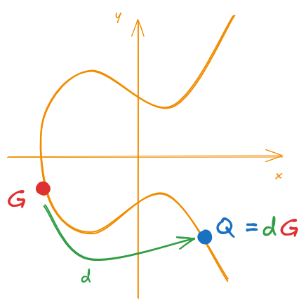
Figure 6: ECDSA Key Generation
Just for the record, recall that:
- Public Key = \(Q\)
- Private Key = \(d\)
Signature Generation (Visual)
With the key generation done, we can now proceed to the “less intuitive” part of the ECDSA… the ECDSA 😅.
If you recall from ECDSA Refresher - Signature Generation, the first step is to generate an ephemeral key \(k_{eph}\) unique for each signature. With this ephemeral key, we generate a new “verification point” \(R\) similar to what we did for the public key:
\begin{equation} \tag{\ref{eq:sig_gen_r}} R = k_{eph} \cdot G \end{equation}
This is illustrated by Figure 7.
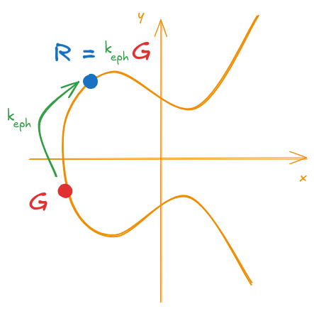
Figure 7: ECDSA generation of the verification point
I’m calling it a “verification point” because, as we will later see, the ECDSA can be thought of as an identification protocol, where we create a “verification value”, and then we provide a proof that will match this “verification value” with some additional steps. This process serves as an assurance that we have knowledge of the private key without exposing it to the verifier (as the majority of signatures schemes do).
For the second part of the signature (the \(s\) part), it is a scalar calculation, so there isn’t much I could show you in terms of making it “visual”. The visual part actually happens at the verification step, just hold on for a bit longer before I show you more images (that’s why you came to this post, right?).
Despite not being a “visual step”, let me dissect a bit the elements that goes in the calculations as they will be useful for us later. Recall that the second part of the signature is generated by Equation \ref{eq:sig_gen_s}:
\begin{equation} \tag{\ref{eq:sig_gen_s}} s \equiv (msg + d \cdot r) \cdot k_{eph}^{-1} \mod{n} \end{equation}
In this equation, the signature is composed by the following components:
- the message: \(msg\) - provides a binding of the generated signature to the message being signed, in other words, if the message changes, the signature should also change.
- the private key: \(d\) - provides a binding of the private key to the signature. This will be important later, as this will assure that the signature will only be valid if using the corresponding public key.
- the x coordinate of R: \(r\) - this is an element that provides a binding between the two parts of the signature. Given that the ECDSA is a signature composed of two parts, we need a way to ensure one cannot modify one part and still generate a valid signature. This is actually a public part of the signature that is included on the second part “as a dependency”. When the verification process occurs, given that this part is public, the verifier will include it in the calculations in a way that they will “cancel out” and everything matches correctly.
- the ephemeral key: \(k_{eph}\) - this is actually one of the core elements of the signature. The ephemeral key is the random key that was used to generate the verification point \(R\). This key is what will allow the verifier to be able to “re-generate” the point “R” using the signature parameters and confirm that the signature is valid. The verification process doesn’t have access to the ephemeral key directly, but it is bundled in the signature in a way that, if every other component of the signature is correct, everything should cancel out, leaving only the ephemeral key behind.
As I already mentioned in some previous sections, since we are using elliptic curves in the real domain, I’ll be taking the poetic license here to interpret the multiplicative inverse as an actual division. Because of that, I’ll now rewrite the Equation \ref{eq:sig_gen_s} as:
\begin{equation} \label{eq:sig_gen_real_domain} s = \frac{msg + d \cdot r}{k_{eph}} \end{equation}
I can then express the final signature as:
\begin{align} Signature &= (r, s) \tag{\ref{eq:sig_tuple}} \ &= \left( r, \frac{msg + d \cdot r}{k_{eph}} \right) \label{eq:sig_tuple_real_domain} \end{align}
Signature Verification (Visual)
The signature verification is where things get interesting and we can better visualize what is actually happening.
Recalling from ECDSA Refresher - Signature Verification, the first three steps are there just to calculate auxiliary values, I’ll be replicating them here just to be easier to reference as I intend to actually expand those values to have a clearer picture of the algorithm.
Equations \ref{eq:aux_value_w}, \ref{eq:aux_value_u1} and \ref{eq:aux_value_u2}, represented below define some auxiliary values used on the verification process:
\begin{gather} w \equiv s^{-1} \mod{n} \tag{\ref{eq:aux_value_w}} \ u_1 \equiv w \cdot msg \mod{n} \tag{\ref{eq:aux_value_u1}} \ u_2 \equiv w \cdot r \mod{n} \tag{\ref{eq:aux_value_u2}} \ \end{gather}
The important part for the verification is actually on the next step, the one represented by Equation \ref{eq:new_point_p_validation}:
\begin{equation} \tag{\ref{eq:new_point_p_validation}} P = u_1 \cdot G + u_2 \cdot Q \end{equation}
In this step, we are calculating a new point \(P\) by using a sum of two other points. If you look closely, the two points we are adding together are:
- a multiple of the base point \(G\)
- a multiple of the public key point \(Q\)
Both points don’t depend on the signature, they are fixed for a given key pair. These points were represented during the key generation step on Figure 6.
What does make this sum different for each signature are the parameters \(u_1\) and \(u_2\) that multiply those base points. Depending on each, the resulting point \(P\) will be located at a completely different place.
Different values of \(u_1\) and \(u_2\) will give us different points, this is illustrated by Figure 8.
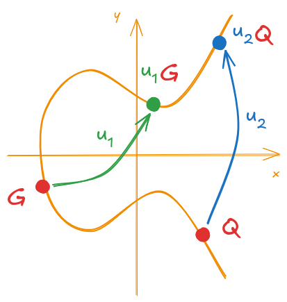
Figure 8: Example of point multiplication for the components of P
With these new points, calculating their sum should result in the point P. This is illustrated on Figure 9.
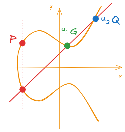
Figure 9: Calculation of the new point P
Now that I think it is clear what we are doing, we need to understand what the \(u_1\) and \(u_2\) are composed of and their relation to the signature.
From Equation \ref{eq:aux_value_u1}:
\begin{equation} u_1 \equiv w \cdot msg \mod{n} \tag{\ref{eq:aux_value_u1}} \ \end{equation}
Since we are using the real domain and not finite fields, I’ll be replacing the “\(\equiv\)” symbol with an “\(=\)” and removing the \(\mod{n}\) to simplify our equations.
Substituting Equations \ref{eq:aux_value_w} and \ref{eq:sig_gen_real_domain}:
\begin{align} u_1 &= w \cdot msg \ &= s^{-1} \cdot msg \ &= \left( \frac{msg + d \cdot r}{k_{eph}} \right)^{-1} \cdot msg \ &= \frac{k_{eph}}{msg + d \cdot r} \cdot msg \label{eq:u_1_expanded_k_eph} \ \end{align}
Just one more step before we proceed, let me make a little change in the representation:
\begin{align} u_1 &= \frac{k_{eph}}{msg + d \cdot r} \cdot msg \tag{\ref{eq:u_1_expanded_k_eph}} \ &= k_{eph} \cdot \frac{msg}{msg + d \cdot r} \label{eq:u_1_expanded_msg} \ \end{align}
Sooo, what do we have here on Equation \ref{eq:u_1_expanded_msg}? If you look closely, we have two elements of a multiplication:
- \(k_{eph}\): the ephemeral key 🤷
- \(\frac{msg}{msg + d \cdot r}\): a fraction with a value less than one
Hold on this information for a bit, let us divert a little to calculate the \(u_2\) before proceeding.
Starting from Equation \ref{eq:aux_value_u2} and using Equations \ref{eq:aux_value_w} and \ref{eq:sig_gen_real_domain}:
\begin{align} u_2 &\equiv w \cdot r \mod{n} \tag{\ref{eq:aux_value_u2}} \ &= s^{-1} \cdot r \ &= \left( \frac{msg + d \cdot r}{k_{eph}} \right)^{-1} \cdot r \ &= \frac{k_{eph}}{msg + d \cdot r} \cdot r \ &= k_{eph} \cdot \frac{r}{msg + d \cdot r} \label{eq:u_2_expanded_msg} \ \end{align}
On Equation \ref{eq:u_2_expanded_msg}, we have a similar pattern from Equation \ref{eq:u_1_expanded_msg}, we have a \(k_{eph}\) and a fraction with a value less than one.
The only difference here is what is on the numerator of the fraction (if you are like me and confuse which one is which, the numerator is the number on top of the fraction 😬). On Equation \ref{eq:u_1_expanded_msg} we had \(msg\) on top, while on Equation \ref{eq:u_2_expanded_msg}, we have \(r\).
This distinction is relevant when we see what value is multiplying which point.
Recalling the Equation \ref{eq:new_point_p_validation}, \(P\) is composed from:
\begin{equation} \tag{\ref{eq:new_point_p_validation}} P = u_1 \cdot G + u_2 \cdot Q \end{equation}
Using our new derived Equations \ref{eq:u_1_expanded_msg} and \ref{eq:u_2_expanded_msg}, we have:
\begin{gather} P = u_1 \cdot G + u_2 \cdot Q \tag{\ref{eq:new_point_p_validation}} \ P = k_{eph} \left( \frac{msg}{msg + d \cdot r} \right) G + k_{eph} \left( \frac{r}{msg + d \cdot r} \right) Q \label{eq:expanded_p_real_domain} \ \end{gather}
Did you see what is going to happen from Equation \ref{eq:expanded_p_real_domain}? We have two points \(G\) and \(Q\), each is being multiplied by \(k_{eph}\) and a fraction. The fraction differs depending on the point being multiplied, one is multiplying the base point, and the other is being multiplied by the public key.
Graphically, we still have the same image, but I’m showing them on Figure 10 just using it to show the expanded constants.
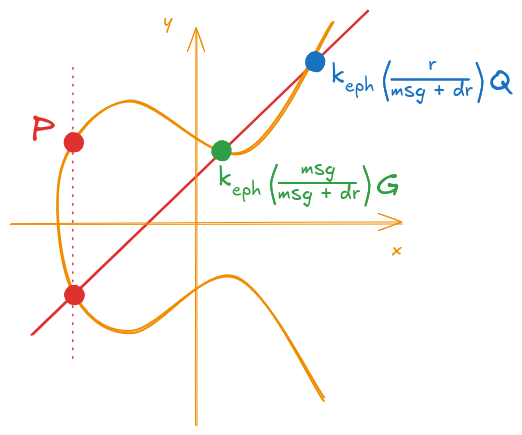
Figure 10: Calculation of the new point P (with expanded auxiliary values)
Finally, from the key generation step, remember from Equation \ref{eq:pub_key_gen} that we have \(Q = d \cdot G\) so Equation \ref{eq:expanded_p_real_domain} turns into:
\begin{align} P &= k_{eph} \left( \frac{msg}{msg + d \cdot r} \right) G + k_{eph} \left( \frac{r}{msg + d \cdot r} \right) Q \tag{\ref{eq:expanded_p_real_domain}} \ &= k_{eph} \left( \frac{msg}{msg + d \cdot r} \right) G + k_{eph} \left( \frac{r}{msg + d \cdot r} \right) (d \cdot G)\ &= k_{eph} \left( \frac{msg}{msg + d \cdot r} \right) G + k_{eph} \left( \frac{d \cdot r}{msg + d \cdot r} \right) G \label{eq:expanded_p_real_domain_private_key}\ \end{align}
Again, its graphical representation is shown on Figure 11.
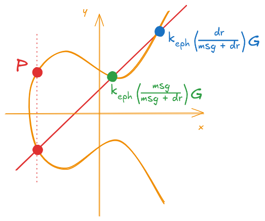
Figure 11: Calculation of the new point P (final expanded form)
If you remember, the validation for the signature is a simple check, see if the verification point \(R\) matches with our newly calculated point \(P\).
Graphically, we just need to confirm if the two points coincide. This is shown on Figures 12 and 13.
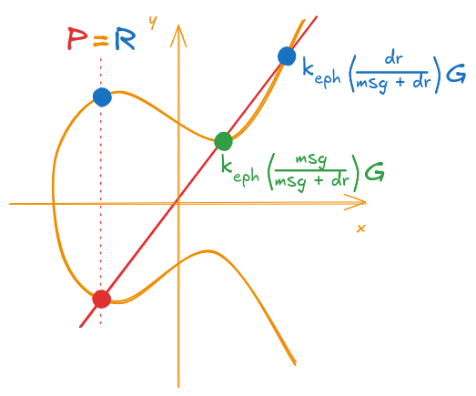
Figure 12: Example of a valid signature (P and R are the same)
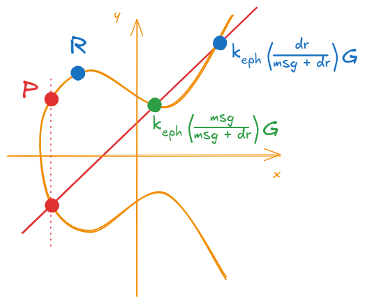
Figure 13: Example of an invalid signature (P and R differ)
Signature Validity (Visual)
Okay, so we know how the points are constructed and when a signature is valid, but what exactly makes a valid signature… valid?
Remember that I said earlier that the ECDSA can be viewed as an identification scheme? What I meant by that was that we are creating a verification point \(R\) and we are giving some additional “hints” that will make the verifier able to arrive to the same point “R”.
The “hints” in question are used on the validation process in such
a way that, if all stars align the parameters are correct, they
should properly cancel out, remaining only the desired value for the
point \(R\).
Before I continue, I should clarify something about the notation in previous sections.
When explaining the signature and verification
processes, I always used the same names for the values being used
(for example the variable msg). However, when we are talking
about signature validity, we need to consider that different parts
of the signature comes at different steps.
For example if we need to consider what an attacker would want to do to forge a signature, he could:
- try to change the message for an already generated signature
- try to generate a valid signature for a key he doesn’t have access to
- try to swap the point
Rto forge a valid signature
And many other possible attacks. To properly analyze when each
scenario could happen, we need to distinguish when each variable of
the signature enters the algorithm. For example, on the first
attack where an adversary would try to find a new message for a
valid signature, the msg parameter during the signature is one
message and the message msg used on the verification process is another.
Assuming the signature process is robust enough (we will show that in a moment), if the message for the signature and verification differs, the signature validation should fail.
To differentiate each value in the process, I’ll be using the following subscripts:
$$X_{key}$$- meaning that the value
Xwas generated during the key generation step $$X_{sig}$$ - meaning that the value
Xwas generated during the signature generation step $$X_{ver}$$ - meaning that the value
Xwas supplied during the signature verification step
As a result, Equation \ref{eq:expanded_p_real_domain} would actually look like the following:
$$P = k_{eph} \left( \frac{msg_{ver}}{msg_{sig} + d_{sig} \cdot r_{sig}} \right) G_{key} + k_{eph} \left( \frac{r_{ver}}{msg_{sig} + d_{sig} \cdot r_{sig}} \right) Q_{key}$$Okay, so let’s start by going back to Equation \ref{eq:expanded_p_real_domain} with the new subscripts (if you don’t know what I’m talking about, please go check the Important box right before this paragraph):
\begin{align} P &= k_{eph} \left( \frac{msg_{ver}}{msg_{sig} + d_{sig} \cdot r_{sig}} \right) G_{key} + k_{eph} \left( \frac{r_{ver}}{msg_{sig} + d_{sig} \cdot r_{sig}} \right) Q_{key} \label{eq:p_with_subscripts} \ \end{align}
Replacing Equation \ref{eq:pub_key_gen} from the key generation step (\(Q_{key} = d_{key} \cdot G_{key}\)):
\begin{align} P &= k_{eph} \left( \frac{msg_{ver}}{msg_{sig} + d_{sig} \cdot r_{sig}} \right) G_{key} + k_{eph} \left( \frac{r_{ver}}{msg_{sig} + d_{sig} \cdot r_{sig}} \right) d_{key} \cdot G_{key} \ &= k_{eph} \left( \frac{msg_{ver}}{msg_{sig} + d_{sig} \cdot r_{sig}} \right) G_{key} + k_{eph} \left( \frac{r_{ver} \cdot d_{key} }{msg_{sig} + d_{sig} \cdot r_{sig}} \right) G_{key} \label{eq:p_expanded_with_subscripts} \ \end{align}
Grouping together similar terms, we have:
\begin{align} P &= k_{eph} \left( \frac{msg_{ver} + d_{key} \cdot r_{ver}}{msg_{sig} + d_{sig} \cdot r_{sig}} \right) G_{key} \label{eq:p_with_grouped_terms} \ \end{align}
If you recall from the verification step, a signature is considered valid if the point \(P\) corresponds to the point \(R\) and. From Equation \ref{eq:sig_gen_r}, we have that \(R = k_{eph} \cdot G\).
The point from Equation \ref{eq:p_with_grouped_terms} will only be equal to \(R\) when the term inside the parenthesis is equal to \(1\) (i.e. we must have \(\left( \frac{msg_{ver} + d_{key} \cdot r_{ver}}{msg_{sig} + d_{sig} \cdot r_{sig}} \right) = 1\)). This will only happen if:
\begin{equation} \label{eq:signature_validity_requirements} \begin{cases} msg_{ver} = msg_{sig} \ d_{key} = d_{sig} \ r_{ver} = r_{sig} \ \end{cases} \end{equation}
If any of these values differ, we wouldn’t have a fraction equal to \(1\) and the signature is considered invalid.
Visually, (with subscripts) we have what’s shown in Figure 14.
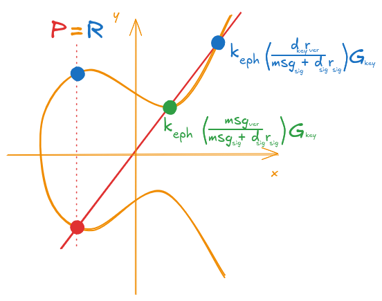
Figure 14: Valid signature visualized with subscripts
But what would happen if any of the values on Equation \ref{eq:signature_validity_requirements} didn’t match? Let’s test some cases.
If an attacker tries to swap the message for an already valid signature, he would try to swap the \(msg_{ver}\). That would make the first term of Equation \ref{eq:p_expanded_with_subscripts} to move away from the correct point (as the \(msg_{ver}\) on the numerator would make the fraction to be “unbalanced” and not equal to 1), which would give an invalid signature. This is shown on Figure 15.
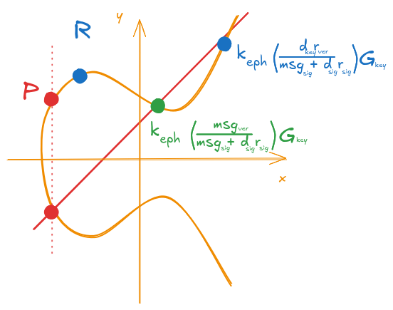
Figure 15: Invalid signature with a message swapped at verification
Another possibility would be for an attacker to try to generate a signature with his keys, but try to send it to be verified with another set of keys. Similarly to the previous case, and assuming that all of the other parameters except the private key get changed, the second term of Equation \ref{eq:p_expanded_with_subscripts} would now move away from the correct position (now the \(d_{sig}\) on the denominator would make the fraction “unbalanced” as the \(d_{key}\) on the numerator is fixed for the public key used on the verification), as shown on Figure 16.
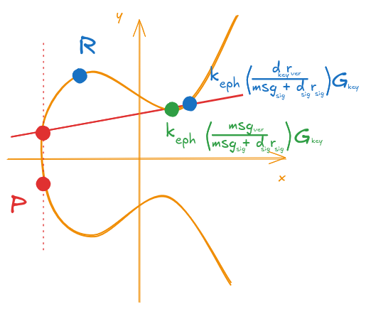
Figure 16: Invalid signature with an invalid private key
I could provide other examples, but I think you might already have an idea of what it would happen. If any parameters gets swapped, corrupted or tweaked, the points (\(P\) and \(R\)) wouldn’t match as the signature process ties together all of the necessary information so that, only when providing the correct parameters, the calculation cancels correctly resulting in the same point.
In a nutshell, a signature can only be considered valid, if all of the correct parameters supplied during the key generation, signature and verification processes matches up. The signature is constructed in a way that it ties all the necessary elements into two components: a “Verification point” \(R\) and a secondary constructed value \(P\) that will only be constructed correctly if we have valid parameters, otherwise the points wouldn’t match.
Conclusion
To summarize this post, let’s recap what the ECDSA does:
- first we generate a keypair by choosing a random private value and then we calculate the corresponding public key
- for the signature, we have two steps:
- generate a random point \(R\) using a random ephemeral key
- generate an “auxiliary value” that “points” to the point \(R\) with additional steps
- for the verification, we:
- use the “auxiliary value” with the other information available (message, public key, point \(R\)) and check that we can “arrive” at the same “point \(R\)” if the signature is correct
If you squint your eyes, this can be seen as a type of an identification protocol.
- we generate a commitment value \(R\)
- then we generate a proof that we know how to arrive on the same \(R\) by using our private key
- if the verification procedure succeeds, that proves that we have the knowledge of the ephemeral key used for \(R\) and that we also have the knowledge of the private key, otherwise the resulting point wouldn’t match.
And that’s pretty much it 🤷.
I hope this post was in any way possible useful to you or anyone trying to get a better intuition over the ECDSA algorithm, if you think it was useful to you, consider sharing it, I would be pretty happy to know that this was useful or educative to someone.
Thank you so much for reaching the end (this post was waaaay bigger than I originally expected), and until my next post (whenever it may be, I need inspiration to do it, who knows when this might happen, perhaps another random chit-chat with other colleagues might bring some ideas 👀).